Two tasks
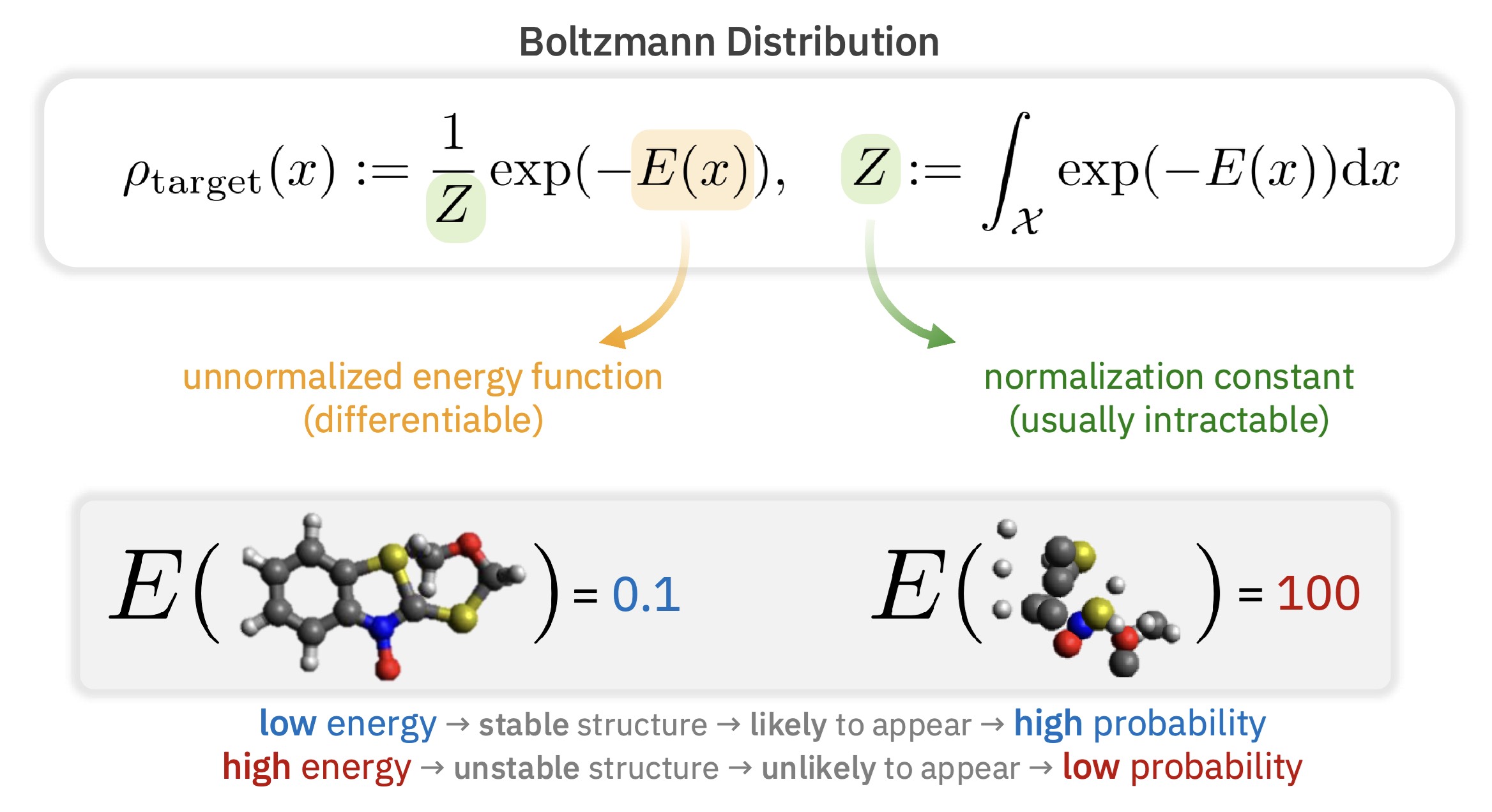
Given an unnormalized probability density function $\pi \propto \hat\pi := \mathrm{e}^{-V}$ on $\mathbb{R}^{d}$:
Draw $X \sim \pi$.
Estimate $Z = \int_{\mathbb{R}^d} \mathrm{e}^{-V(x)}\,\mathrm{d}x$, or equivalently, the free energy $F = -\log Z$.
Applications: Bayesian posteriors & evidence; the partition function / free energy in statistical mechanics; energy-based & latent-variable models; volume of convex bodies.
They look like two problems — I'll argue they're closely related, and the same number tells you how hard both are.
Why we care
Where these show up
The same $\pi\propto\mathrm{e}^{-V}$ shows up across domains:
Statistical mechanics / molecular dynamics
(Figure: Guan-Horng Liu's talk on ASBS.)
Bayesian inference
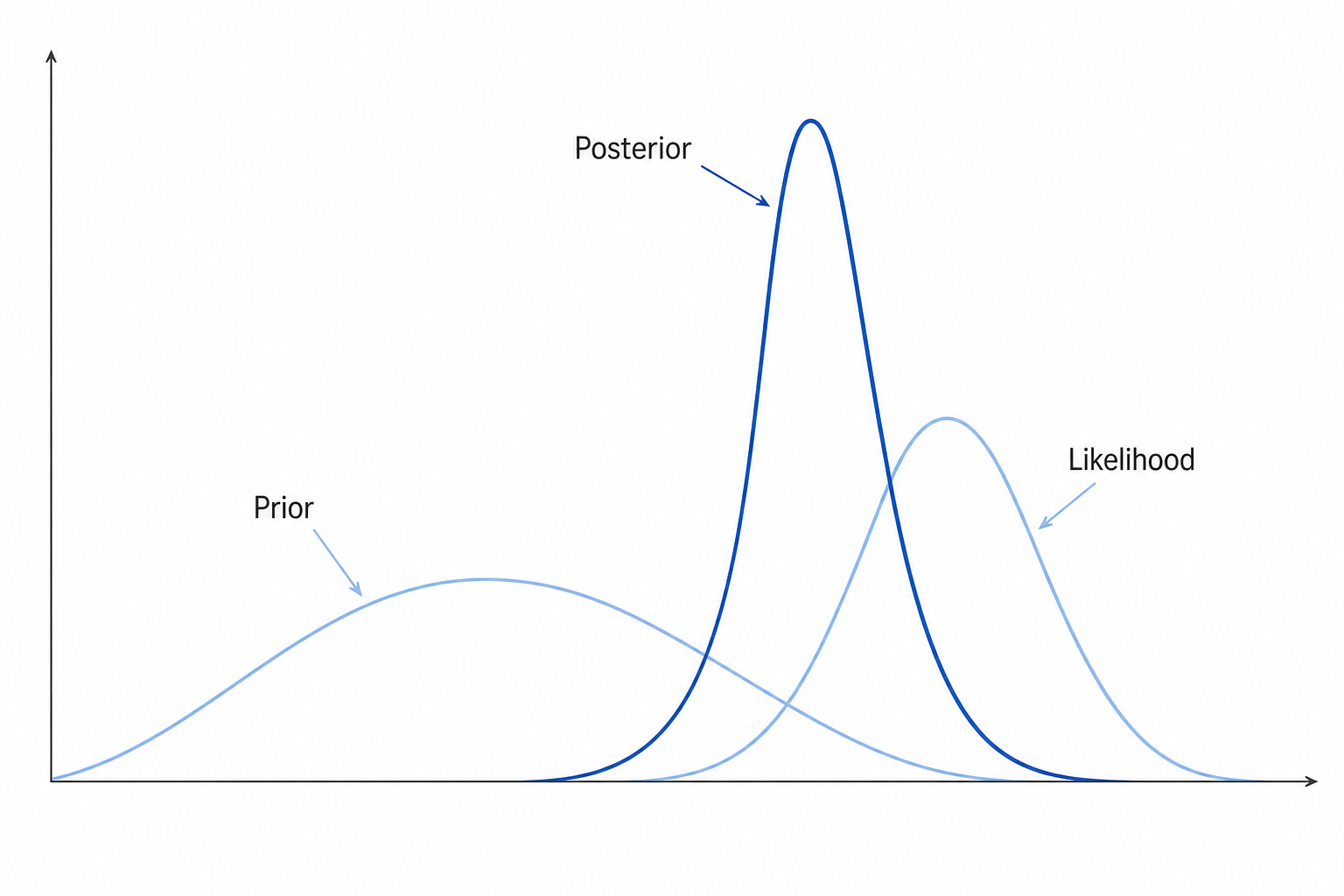
unnormalized = likelihood $\times$ prior; $Z=p(\mathcal{D})$ = evidence (marginal likelihood).
Sampling $\leftrightarrow$ configurations / posterior samples; normalizing constant $\leftrightarrow$ free energy / model evidence.
Background
The classical recipes
Each task has a classical approach:
Build a Markov chain whose stationary law is $\pi$ (Metropolis–Hastings, Gibbs, Langevin, …) and run the chain till convergence.
With a tractable proposal $\pi_0$: $Z = \mathbb{E}_{\pi_0}\!\left[\frac{\hat\pi}{\pi_0}\right] \approx \frac1n\sum_{i=1}^n \frac{\hat\pi(X_i)}{\pi_0(X_i)}$, $X_i\sim\pi_0$.
Clean and provably efficient when $\pi$ is well-conditioned, or close to $\pi_0$.
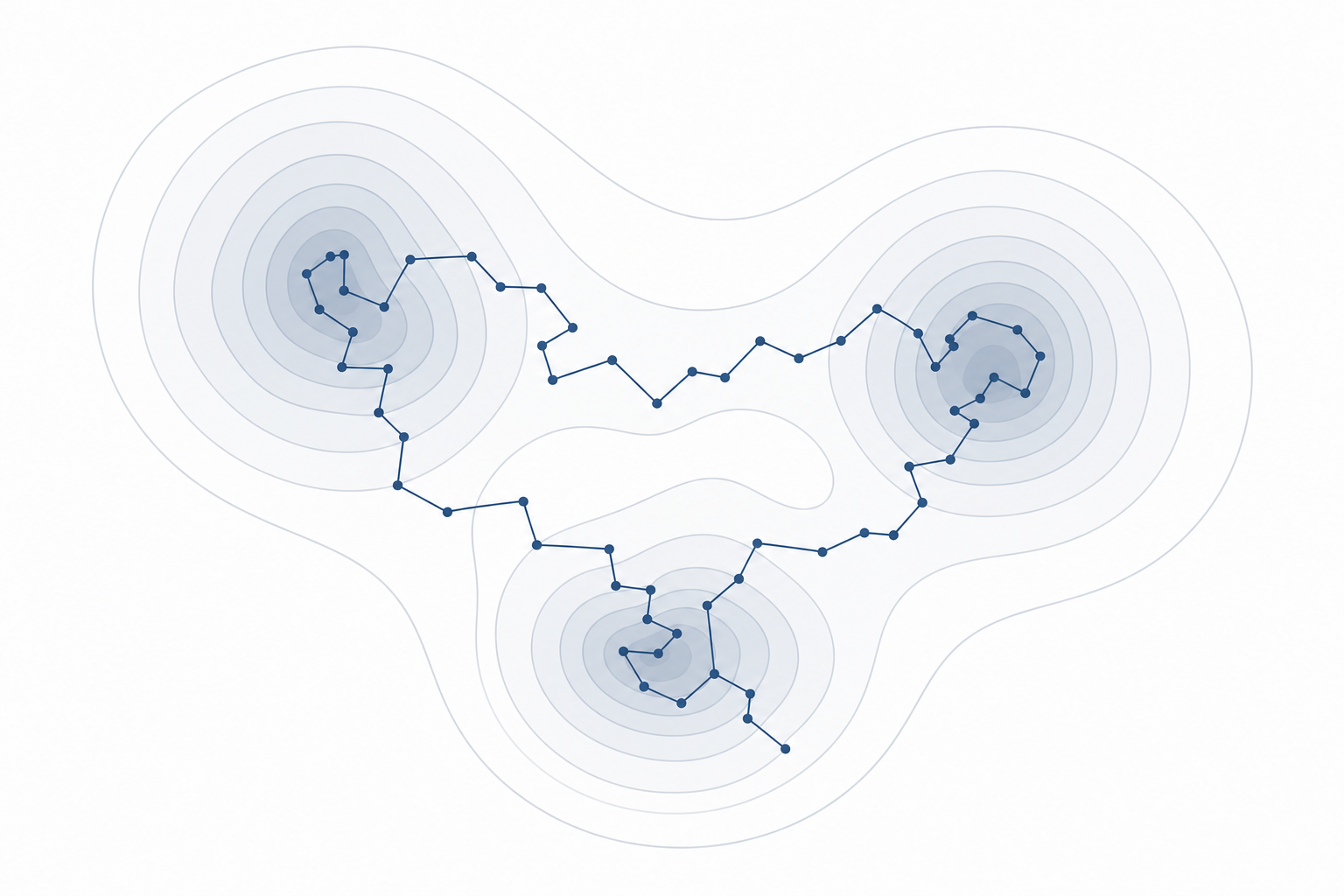
Why it's hard in practice
Plain Langevin / MCMC gets trapped in one mode $\Rightarrow$ mixing time exponential in mode distance / dimension.
Naive importance sampling has high variance from proposal–target mismatch.
High dimension + multimodality is the shared difficulty.
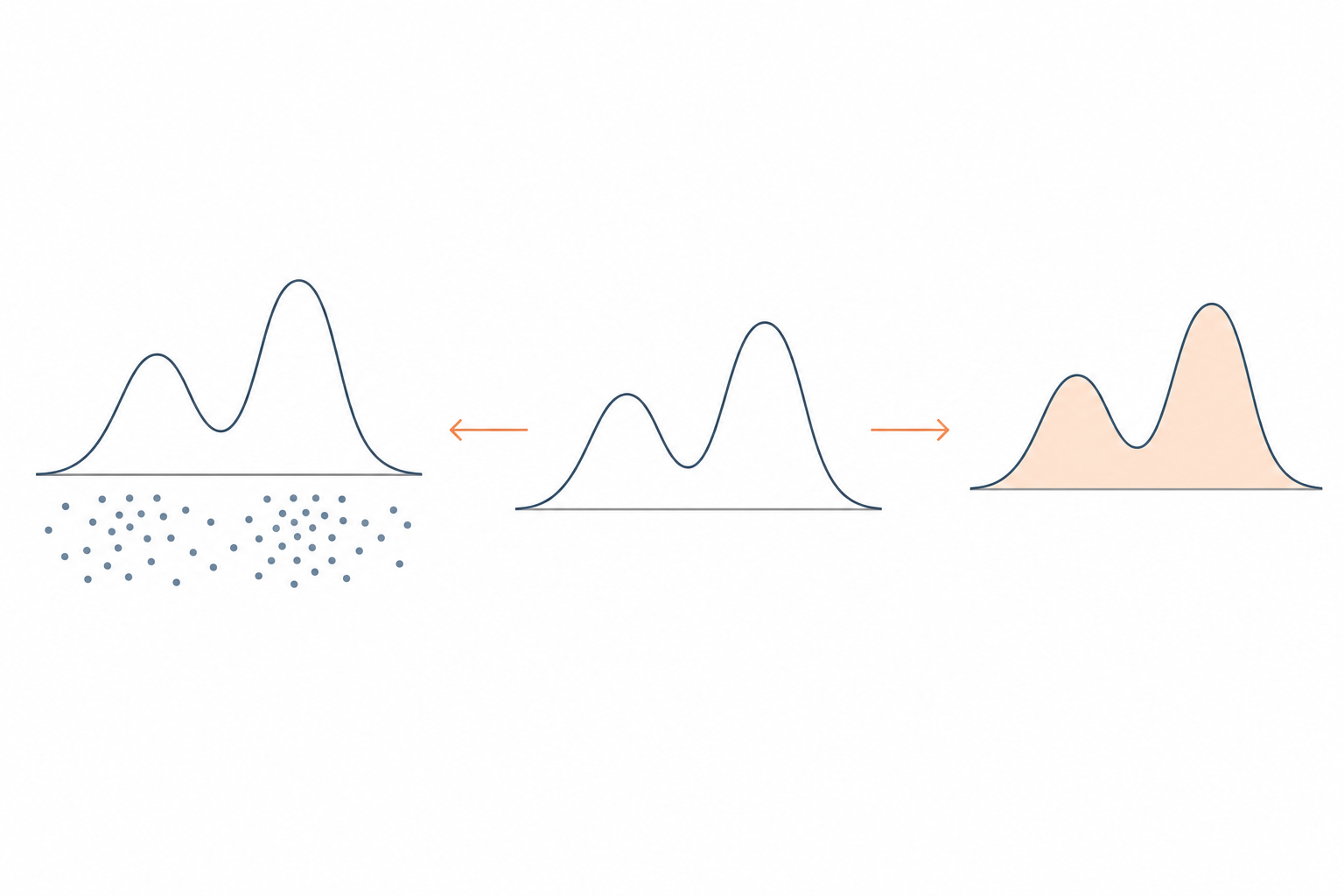
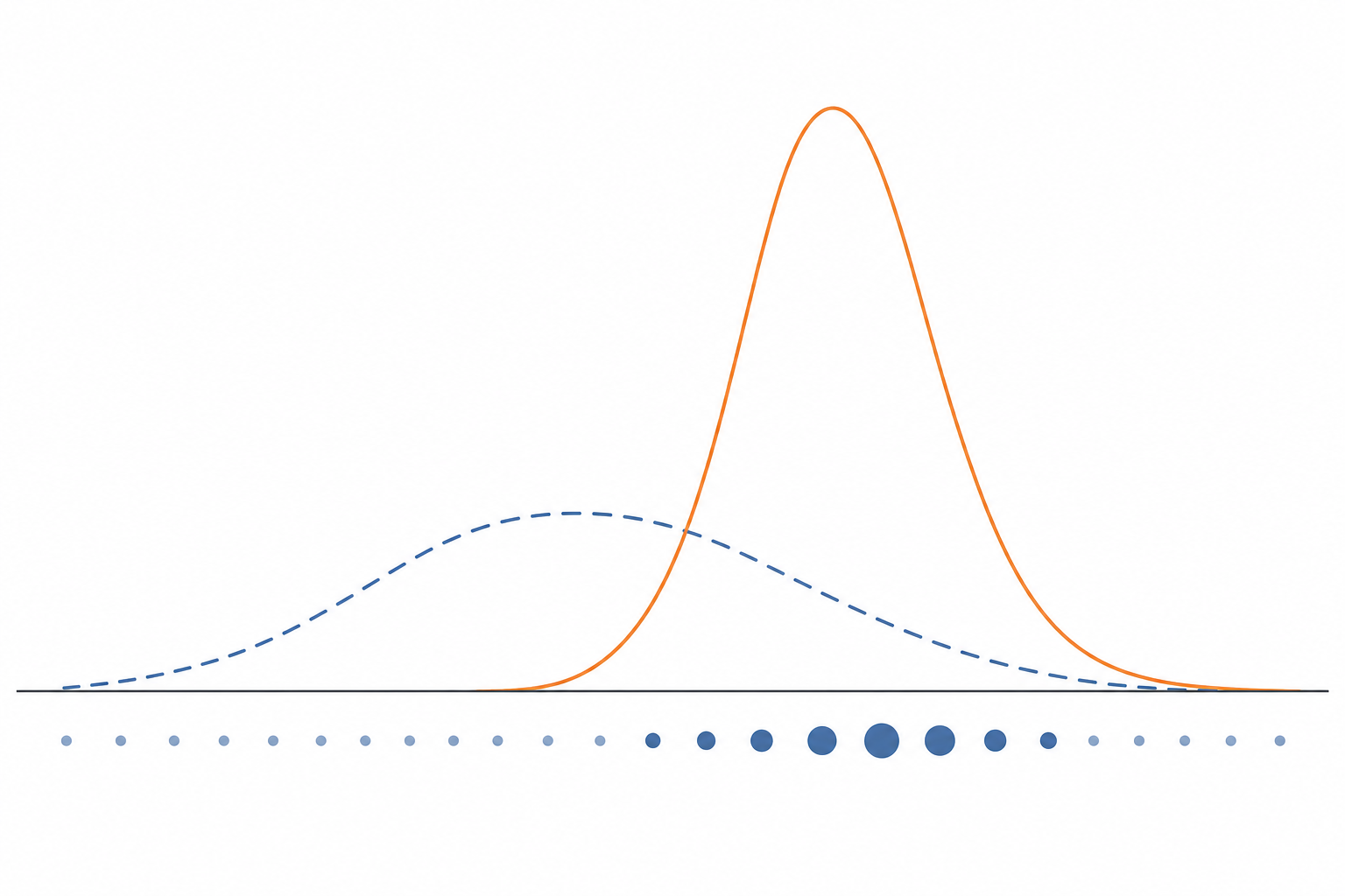
Annealing: a smooth interpolation between distributions
Bridge $\pi_0 \to \pi$ with a curve of distributions
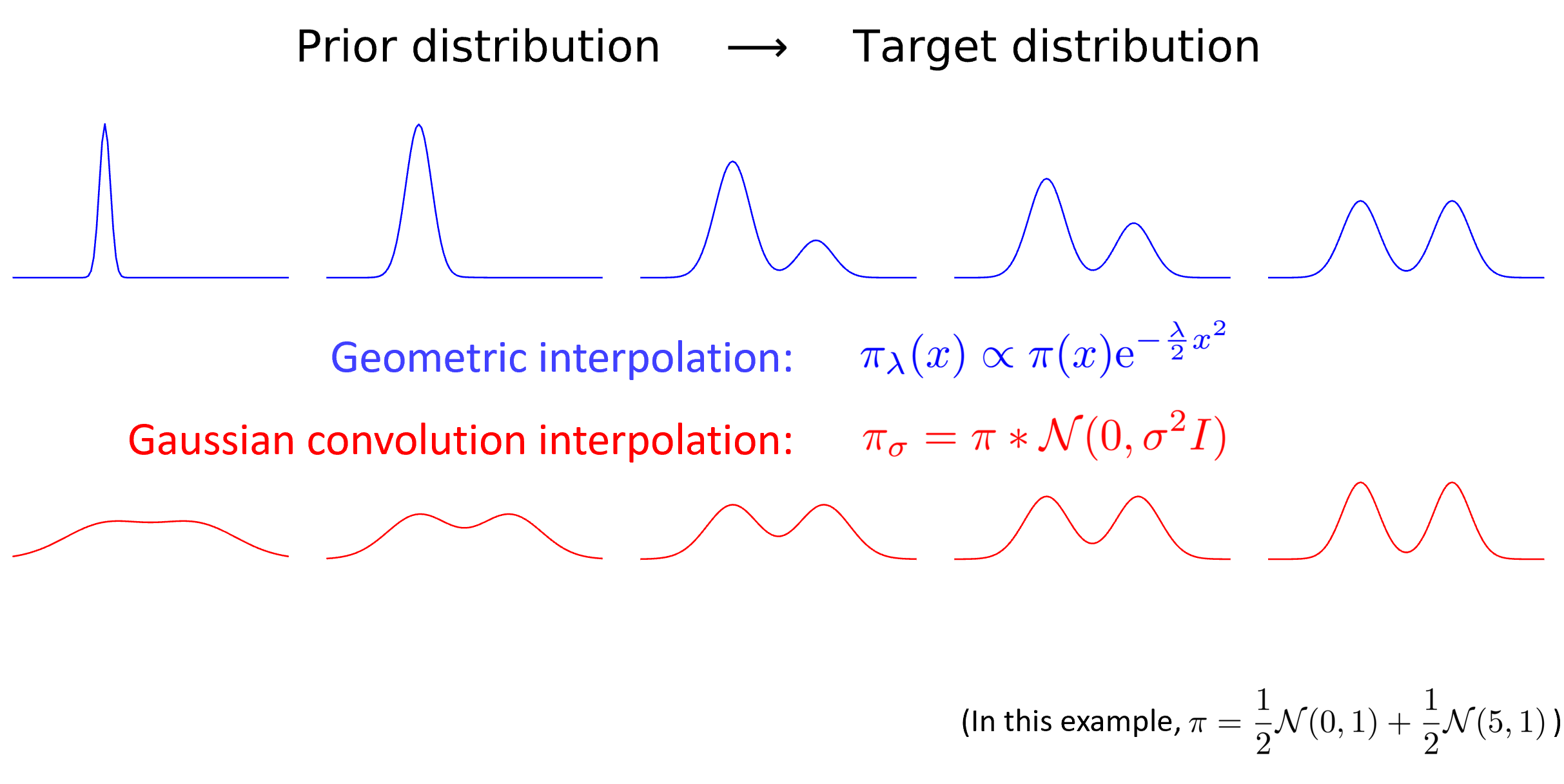
Two common choices:
- Geometric: $\pi_\theta \propto \exp\!\big(-V - \frac{\lambda(\theta)}{2}\|\cdot\|^2\big)$.
- Gaussian convolution: $\pi_\theta = \pi * \mathcal{N}\!\big(0,\sigma(\theta)^2 I\big)$.
Replace one hard jump with many easy steps — break the hard problem down along the curve.
The toolkit
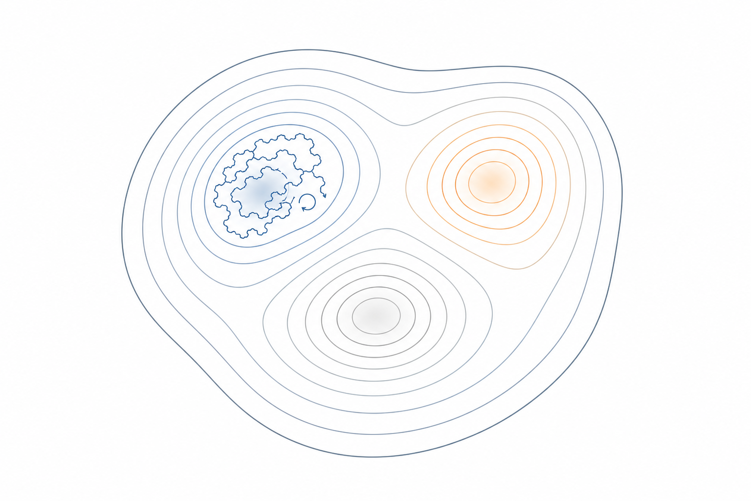
Optimal transport
- Curve “speed” = Wasserstein-2 metric derivative $|\dot\rho|_t := \lim_{\delta\to0}\frac{W_2(\rho_{t+\delta},\rho_t)}{|\delta|}$.
- Continuity equation: a vector field $(v_t)$ generates $(\rho_t)$ iff $\partial_t\rho_t + \nabla\!\cdot(\rho_t v_t)=0$. Equivalently, if $\dot X_t = v_t(X_t)$ and $X_0 \sim \rho_0$, then $X_t \sim \rho_t$.

Optimal transport. (Figure: Wikipedia)
Ambrosio, Gigli & Savaré (2008), Gradient Flows: In Metric Spaces and in the Space of Probability Measures.
The big picture
The proof idea: three path measures
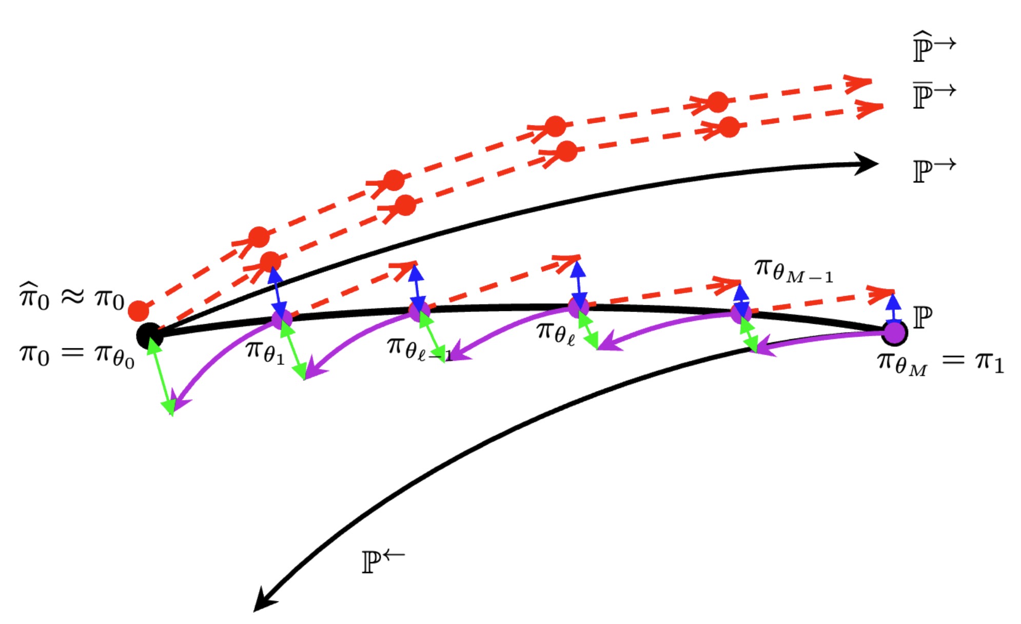
Forward $\mathbb{P}^{\rightarrow}$ (the algorithm), backward $\mathbb{P}^{\leftarrow}$, and the compensated reference $\mathbb{P}$ threading the intermediates $\pi_{\theta_\ell}$.
Beyond geometric interpolation
The catch with geometric interpolation
- The whole story hinges on $\mathcal{A}$ being small, but it need not be.
- 1-dimensional example: $\pi = \frac12\mathcal{N}(0,1)+\frac12\mathcal{N}(m,1)$, $\pi_\theta(x)\propto\pi(x)\,\mathrm{e}^{-\lambda(\theta)x^2/2}$, $\lambda(\theta)=m^2(1-\theta)^r$.
exponential in the mode separation
Mass teleportation / Mode switching: weights of the modes change dramatically, so mass must teleport across a large distance.
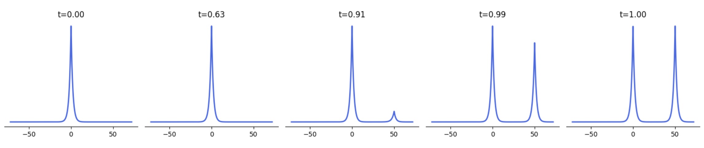
Figure: Chemseddine, Wald, Duong & Steidl (2025), Neural Sampling from Boltzmann Densities: Fisher–Rao Curves in the Wasserstein Geometry, ICLR.